Viscoelastic Fluid Flows
1 Table of contents
🔬 Key Topics:
2 Overview
2.1 The challenges of simulating viscoelastic flows
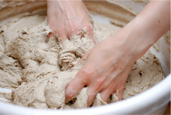
Viscoelastic fluids are a special type of non-Newtonian fluid, a kind of materials whose behavior changes depending on the forces applied to them. What makes these fluids truly fascinating is that they can act both like regular liquids, flowing and adapting, and like solids that resist and hold their shape… all depending on how fast or how strongly they are deformed.
Here you can see a fun experiment carried out at Lamar University (USA), where a small swimming pool was filled with a non-Newtonian fluid. The students were even able to walk on the surface, but only as long as they kept moving!
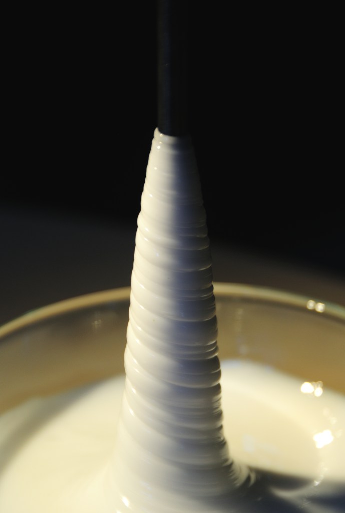
More specifically, viscoelastic fluids exhibit both viscous (frictional, dissipative) and elastic (energy-storing, memory-retaining) behaviors. This unique combination arises from their complex internal microstructure, which leads to memory effects:
The current stress state depends not only on the present deformation but also on the entire flow history.
Therefore, accurately model these fluids is not simple: one must go beyond the classical Navier–Stokes equations and employ nonlinear constitutive equations. This complexity makes the numerical simulation of viscoelastic fluid flows especially challenging, particularly at high Weissenberg numbers, which correspond to flows dominated by elastic effects.

This is in fact one of the biggest challenges in computational rheology, dating back to the 1970s called High Weissenberg Number Problem (HWNP). At that time, all methods were observed to break down at relatively low Weissenberg numbers. For approximately 30 years, this breakdown was believed to be a purely numerical phenomenon.
This research area started from my PhD work and focuses on the numerical simulation of these complex flows using the Finite Element Method (FEM). The goal is to develop stable and accurate numerical techniques to better understand and predict the behavior of viscoelastic fluids with high elasticity across a wide range of applications, from industrial processes to biological systems.
The numerical developments were implemented in the in-house FEM code Femuss. The code allows for modular addition of constitutive models, solver schemes, and stabilization techniques.
2.2 Modelling of polymeric fluid flows
While Newtonian fluids can be modeled using only the Navier–Stokes equations (which include the momentum and continuity equations), modeling viscoelastic fluid flows requires a nonlinear constitutive equation to properly capture the elastic behavior of the fluid.
where the unknowns are the velocity \(\boldsymbol{u}\), pressure \(p\) and the extra stress tensor \(\boldsymbol{\sigma}\). The Deviatoric stress tensor is denoted by \(\mathbf{T}\), \(\eta_p\) is the polymer viscosity coefficient and \(\lambda\) is the relaxation time. The expression of \(\mathfrak{h}(\boldsymbol{\sigma})\) depends on the model chosen. In general \(\mathfrak{h}(\boldsymbol{\sigma})=0\), which corresponds to the Oldroyd-B model.
Also, note that \(\mathbf{T}\) adopts different forms, depending of the fluid flow to simulate:
Newtonian viscous fluids: \(\mathbf{T} = 2 \eta \nabla^s \boldsymbol{u}\)
Polymeric fluids: \(\mathbf{T} = 2 \eta_s \nabla^s \boldsymbol{u} + \boldsymbol{\sigma}\)
where \(\eta_s\) is the solvent viscosity for viscoelastic fluid flows. Note that \(\eta_s+\eta_p=\eta\), that is the usual viscosity employed for Newtonian fluids.
2.3 The Weissenberg Number
The Weissenberg number (We) is a dimensionless quantity that compares elastic and viscous effects in viscoelastic fluid flows. It is defined as:
\[ \mathrm{We} = \frac{\lambda U}{L} \]
Where \(\lambda\) is relaxation time, \(U\) is the characteristic velocity and \(L\) characteristic length.
The physical interpretation is:
- If \(\mathrm{We}\) is small: Viscous effects dominate, elastic behavior is negligible.
- If \(\mathrm{We}\) is large (typically \(\mathrm{We} > 1\)): Elastic effects become significant, leading to complex flow behavior and numerical difficulties.
2.4 Weak Formulation
The weak form of the problem consists in finding \(\boldsymbol{U} = [\boldsymbol{u}, p, \boldsymbol{\sigma}] : ]0, t_{\rm f}[ \longrightarrow \boldsymbol{\mathcal{X}} := \boldsymbol{\mathcal{V}}_0 \times \boldsymbol{\mathcal{Q}} \times \boldsymbol{\Upsilon}\), such that the initial conditions are satisfied and:
\[ \left(\rho \dfrac{\partial \boldsymbol{u}}{\partial t}, \boldsymbol{v}\right) + (\boldsymbol{\sigma}, \nabla^{s} \boldsymbol{v}) + 2 (\eta_{s} \nabla^{s} \boldsymbol{u}, \nabla^{s} \boldsymbol{v}) + \langle \rho \boldsymbol{u} \cdot \nabla \boldsymbol{u}, \boldsymbol{v} \rangle - (p, \nabla \cdot \boldsymbol{v}) = \langle \boldsymbol{f}, \boldsymbol{v} \rangle, \] \[ (q, \nabla \cdot \boldsymbol{u}) = 0, \] \[ \dfrac{1}{2 \eta_{p}} (\boldsymbol{\sigma}, \boldsymbol{\chi}) - (\nabla^{s} \boldsymbol{u}, \boldsymbol{\chi}) + \dfrac{\lambda}{2 \eta_{p}} \left( \dfrac{\partial \boldsymbol{\sigma}}{\partial t} + \boldsymbol{u} \cdot \nabla \boldsymbol{\sigma} - \boldsymbol{\sigma} \cdot \nabla \boldsymbol{u} - (\nabla \boldsymbol{u})^{T} \cdot \boldsymbol{\sigma}, \boldsymbol{\chi} \right) = 0, \]
for all \(\boldsymbol{V} = [\boldsymbol{v}, q, \boldsymbol{\chi}] \in \boldsymbol{\mathcal{X}}\), where it is assumed that \(\boldsymbol{f}\) is such that \(\langle \boldsymbol{f}, \boldsymbol{v} \rangle\) is well defined.
In compact form, the problem can be written as:
\[ \mathcal{G}(\boldsymbol{U}, \boldsymbol{V}) + B(\boldsymbol{u}; \boldsymbol{U}, \boldsymbol{V}) = L(\boldsymbol{V}),\]
for all \(\boldsymbol{V} \in \boldsymbol{\mathcal{X}}\), where:
\(\mathcal{G}(\boldsymbol{U}, \boldsymbol{V}) = \left(\rho \dfrac{\partial \boldsymbol{u}}{\partial t}, \boldsymbol{v}\right) + \dfrac{\lambda}{2 \eta_{0}} \left(\dfrac{\partial \boldsymbol{\sigma}}{\partial t}, \boldsymbol{\chi} \right),\)
\(\begin{aligned} B(\hat{\boldsymbol{u}}; \boldsymbol{U}, \boldsymbol{V}) =\ & 2 (\eta_{s} \nabla^{s} \boldsymbol{u}, \nabla^{s} \boldsymbol{v}) + \langle \rho \hat{\boldsymbol{u}} \cdot \nabla \boldsymbol{u}, \boldsymbol{v} \rangle + (\boldsymbol{\sigma}, \nabla^{s} \boldsymbol{v}) \\ & - (p, \nabla \cdot \boldsymbol{v}) + (q, \nabla \cdot \boldsymbol{u}) + \dfrac{1}{2 \eta_{p}} (\boldsymbol{\sigma}, \boldsymbol{\chi}) - (\nabla^{s} \boldsymbol{u}, \boldsymbol{\chi}) \\ & + \dfrac{\lambda}{2 \eta_{p}} \left( \hat{\boldsymbol{u}} \cdot \nabla \boldsymbol{\sigma} - \boldsymbol{\sigma} \cdot \nabla \hat{\boldsymbol{u}} - (\nabla \hat{\boldsymbol{u}})^{T} \cdot \boldsymbol{\sigma}, \boldsymbol{\chi} \right), \end{aligned}\)
\(L(\boldsymbol{V}) = \langle \boldsymbol{f}, \boldsymbol{v} \rangle.\)
2.5 Spatial discretization using the Finite Element Method
The Galerkin finite element method consists in seeking an approximate solution within a finite-dimensional subspace of the original infinite-dimensional function space. Given a weak formulation of the problem, the solution is approximated by projecting it onto a finite element space constructed from piecewise polynomial basis functions defined over a mesh of the computational domain.
In this framework, the trial and test functions are chosen from the same finite element space, ensuring consistency and stability under appropriate conditions.
In general, the finite element partition of the domain \(\Omega\) is denoted by \(\mathcal{T}_{h} = \{K\}\). Likewise, the diameter of an element \(K \in \mathcal{T}_{h}\) is denoted by \(h_{K}\), and the diameter of the partition is defined as \(h = \max\{h_{K} \mid K \in \mathcal{T}_{h}\}.\) From \(\mathcal{T}_{h}\) we construct conforming finite element spaces for the velocity, the pressure, and the elastic stress: \(\boldsymbol{\mathcal{V}}_{h} \subset \boldsymbol{\mathcal{V}}\), \(\mathcal{Q}_{h} \subset \mathcal{Q}\), and \(\boldsymbol{\Upsilon}_{h} \subset \boldsymbol{\Upsilon}\), respectively.
Therefore, defining \(\boldsymbol{\mathcal{X}}_{h} := \boldsymbol{\mathcal{V}}_{h} \times \mathcal{Q}_{h} \times \boldsymbol{\Upsilon}_{h},\) the Galerkin finite element approximation of the standard problem consists in finding \(\boldsymbol{U}_{h} : ]0, t_{\mathrm{f}}[ \longrightarrow \boldsymbol{\mathcal{X}}_{h},\) such that:
\[ \underbrace{\mathcal{G}(\boldsymbol{U}_{h}, \boldsymbol{V}_{h})}_{\text{Temporal terms}} + \underbrace{B(\boldsymbol{u}_{h}; \boldsymbol{U}_{h}, \boldsymbol{V}_{h})}_{\text{Bilinear form}} = L(\boldsymbol{V}_{h}), \]
for all \(\boldsymbol{V}_{h} \in \boldsymbol{\mathcal{X}}_{h}\).
The resulting system is a set of algebraic equations that can be efficiently solved using numerical linear algebra techniques.
2.6 Stabilization
In incompressible flow problems, using equal-order interpolation for velocity and pressure in finite element methods often leads to numerical instabilities due to the violation of the inf-sup (or Ladyzhenskaya–Babuška–Brezzi) condition. This condition is essential to ensure the well-posedness of the continuous and discrete problems, namely the existence and uniqueness of the solution.
To address this, stabilization techniques are introduced, modifying the formulation slightly to recover stability without compromising accuracy. Among the various available strategies, we adopt the Variational Multiscale (VMS) method. VMS techniques are robust, residual-based, and provide a systematic framework that enhances stability and ensures mesh-convergent solutions.
The key idea in Variational Multiscale Methods (VMS) is to decompose the solution and test space into coarse (resolved) and fine (unresolved) scales: \[ \boldsymbol{U} = \boldsymbol{U}_h + \boldsymbol{U}', \quad \boldsymbol{V} = \boldsymbol{V}_h + \boldsymbol{V}', \] where \(\boldsymbol{U}_h, \boldsymbol{V}_h \in \boldsymbol{\mathcal{X}}_{h}\) (finite-dimensional space), and \(\boldsymbol{U}', \boldsymbol{V}' \in \boldsymbol{\mathcal{X}}'\) (the complementary fine-scale space).
Inserting the decomposition into the variational formulation and requiring it to hold for all \(\boldsymbol{V}_h \in \boldsymbol{\mathcal{X}}_{h}\) and \(\boldsymbol{V}' \in \boldsymbol{\mathcal{X}}'\), we obtain a coupled system for the resolved and unresolved scales. Then, the fine scales \(\boldsymbol{U}'\) are approximated (typically in terms of the residual of the coarse-scale equation), leading to a modified coarse-scale problem of the form: \[ \mathcal{G}(\boldsymbol{U}_{h}, \boldsymbol{V}_{h})+B(\boldsymbol{u}_h;\boldsymbol{U}_h, \boldsymbol{V}_h) + S(\boldsymbol{U}_h, \boldsymbol{V}_h) = L(\boldsymbol{V}_h) \quad \forall \boldsymbol{V}_h \in \boldsymbol{\mathcal{X}}_{h}, \] where the stabilization operator \(S(\cdot, \cdot)\) accounts for the effect of the unresolved scales.
This framework provides a systematic and physically motivated way to derive stabilized formulations, especially effective for problems with dominant advection or incompressibility constraints.
3 Logarithmic Conformation Reformulation
📄 Moreno, L., Codina, R., Baiges, J., & Castillo, E. (2019).
Logarithmic conformation reformulation in viscoelastic flow problems approximated by a VMS-type stabilized finite element formulation.[Post-print]
Computer Methods in Applied Mechanics and Engineering, 354, 706–731.
DOI: 10.1016/j.cma.2019.06.001
As mentioned in the overview, one of the main challenges in computational rheology is the simulation of viscoelastic fluid flows at high elasticity. This issue, commonly referred to as the High Weissenberg Number Problem (HWNP), severely limits the range of applicability of numerical methods in viscoelastic flow simulations.
3.1 Main Concepts
In 2004, Fattal and Kupferman provided a key insight by identifying two main sources of instability associated with this problem:
Inadequate approximations for representing the polymeric stress tensor, which can lead to unphysical results or numerical blow-up.
The requirement to preserve the positive-definiteness of the conformation tensor. This tensor, denoted by \[ \boldsymbol{\tau} = \lambda \dfrac{\boldsymbol{\sigma}}{\eta_p} + \mathbf{I} \] must remain positive-definite to ensure physically meaningful solutions. However, standard discretization techniques may violate this condition, leading to instabilities in the numerical simulation.
These findings laid the groundwork for the development of more robust numerical schemes, such as the Log-conformation Reformulation (LCR), which aim to overcome these difficulties by reformulating the constitutive equations in a way that inherently preserves the mathematical and physical properties of the model. Therefore, Fattal and Kupferman proposed a reformulation that is essentially a change of variables. The original formulation by Fattal and Kupferman considers the next transformation:
\[ \boldsymbol{\psi} = \log\left( \dfrac{\lambda \boldsymbol{\sigma}}{\eta_p} + \mathbf{I} \right) \] This change of variables ensure the conformation tensor remains physically admissible, which requires it to be symmetric and positive-definite at all times.
Following this important discovery, we apply the same change of variables, with some modifications to suit our model:
\[ \boldsymbol{\psi} = \log\left(\boldsymbol{\tau}\right) = \log\left( \dfrac{\lambda_0 \boldsymbol{\sigma}}{\eta_p} + \mathbf{I} \right) \quad \longrightarrow \quad \boldsymbol{\sigma} = \dfrac{\eta_p}{\lambda_0} \left( \exp(\boldsymbol{\psi}) - \mathbf{I} \right) \]
where, \(\lambda_0 = \max\{k\lambda, \lambda_{0,\min}\}\).
Note: Unlike the original change of variables, our formulation is non-singular when the Weissenberg number \(\mathrm{We}\) tends to zero, avoiding potential numerical issues in this limit.
By substituting this reformulated variable \(\boldsymbol{\psi}\) into the original governing equations, we obtain a new system of equations where the primary unknowns are the velocity \(\boldsymbol{u}\), the pressure \(p\), and the transformed tensor \(\boldsymbol{\psi}\).
Considering this new system, we develop a Variational Multiscale (VMS) stabilization strategy for stabilize the reformulated problem. Moreover, we design a “split” type stabilization method, which focuses on the essential terms necessary to stabilize the problem efficiently, while still achieving optimal convergence rates.
This approach significantly improves the robustness and accuracy of the numerical simulations for viscoelastic flows at high Weissenberg numbers.
3.2 Numerical Results
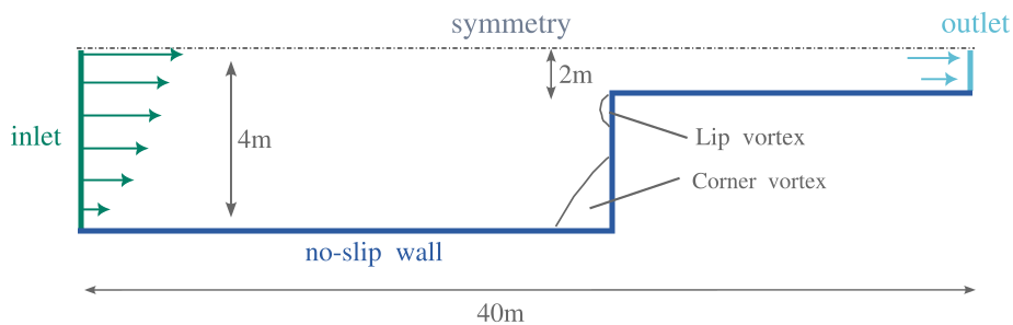
Contraction 4:1
This benchmark is widely used to test the performance of numerical methods in viscoelastic fluid simulations. It features a planar channel with a 4:1 contraction, which produces strong elastic effects at high Weissenberg numbers. The goal is to evaluate the stability and accuracy of the numerical approach under demanding flow conditions, and to compare the results with reference data from the literature.
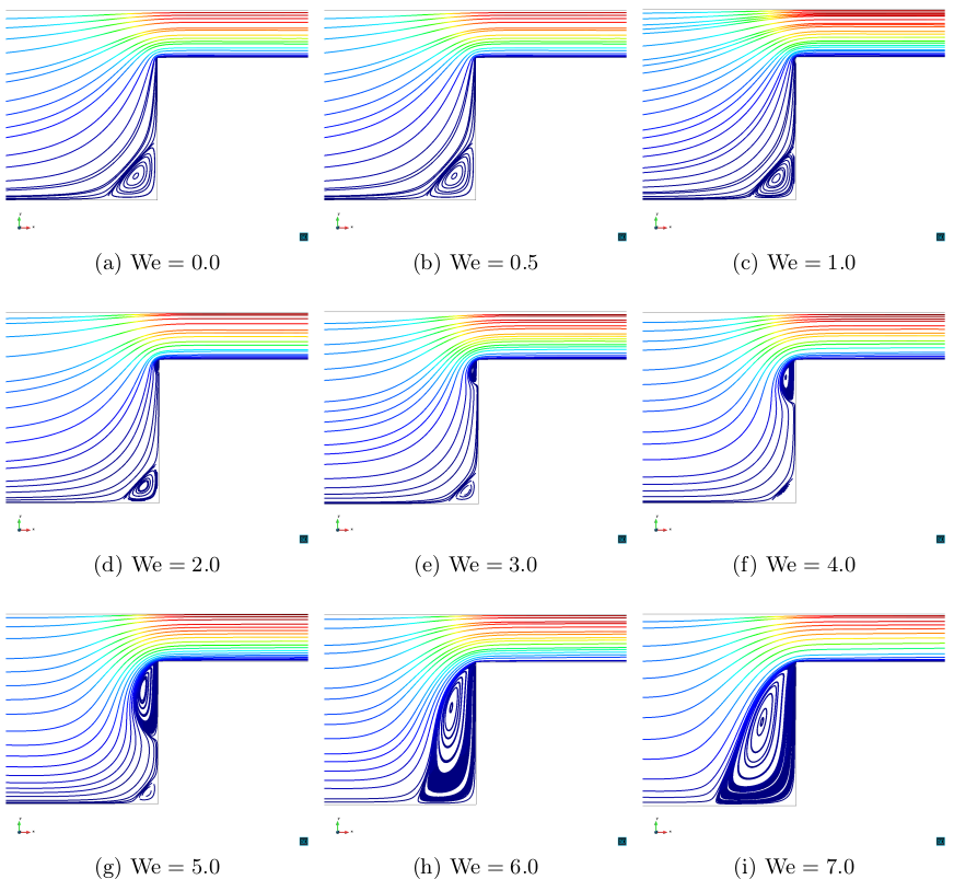
The following images show the streamlines of the fluid flow inside the channel. Before diving into the explanations, I’d like to apologize to the reader for the terrible color choices. I have no excuse… but in my defense, I was in the first year of my PhD! That said, it’s important to clarify that the problem has a stationary solution. Each image corresponds to a different simulation with a different fluid, but all of them share the same Reynolds number, Re = 1.
Recall that the Weissenberg number (We) indicates the elasticity of the fluid flow. The image labeled We = 0 corresponds to a viscous Newtonian fluid with no elasticity. As the Weissenberg number increases, we can observe how the behavior of the streamlines changes for each elastic fluid. This study allows us to analyze the length and shape of the vortex across different elastic regimes.
Beyond capturing the expected behavior, one key point should be highlighted: standard formulations (i.e., without any change of variables) typically struggle to simulate beyond We = 2.5. In contrast, our formulation (combined, of course, with the developed stabilization strategy) demonstrates robustness in simulating highly elastic flows, which was the main goal of this work.
Finally, the size of the bottom corner vortex is compared with results from the literature for fluids with We ≤ 5. M3 indicates the results obtained in this study (for more details, feel free to check out the paper).
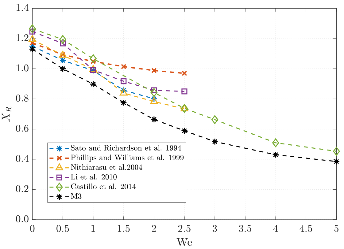
3.3 Conclusions
To sum up, the method (change of variables + VMS stabilization developed) shows good agreement with the literature, performs robustly for high Weissenberg numbers, and captures the main features of the flow. Not bad for a first PhD paper, right?
4 Thermal Coupling
📄 Moreno, L., Codina, R., & Baiges, J. (2021).
Numerical simulation of non-isothermal viscoelastic fluid flows using a VMS stabilized Finite Element formulation. Post-print
Journal of Non-Newtonian Fluid Mechanics, 296, 104640.
DOI: 10.1016/j.jnnfm.2021.104640
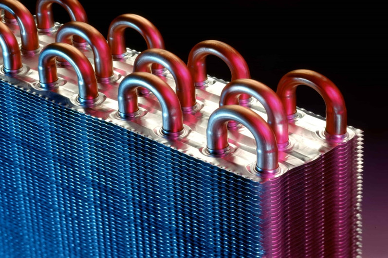
This second key topic seeks to explore how temperature variations affect the behavior of viscoelastic fluid flows. Viscoelastic fluids exhibit highly advantageous properties for heat transfer and energy transport processes. In many industrial applications, such as polymer extrusion or heat exchangers, these fluids are capable of converting significant amounts of mechanical energy into heat due to their complex rheological behavior.
Therefore, this study aimed to shedding light on the coupling between thermal and mechanical effects in non-isothermal conditions. These insights are not only relevant in classical industrial settings, but also open the door to emerging applications such as solar thermal systems, where enhanced heat transfer performance is key to improving efficiency.
4.1 Main Concepts
In non-isothermal viscoelastic fluids, the stress no longer depends solely on the deformation and its history, as is the case in isothermal models. Instead, it is also influenced by the temperature and its temporal evolution. This adds a new layer of complexity to the modeling, as both the thermal and mechanical histories must be taken into account.
Now, the parameters used in viscoelastic models, such as the solvent and polymeric viscosities \(\eta_s\), \(\eta_p\), and the relaxation time \(\lambda\), become temperature-dependent. This dependence is commonly modeled using the principle of time-temperature superposition, twhich provides a way to relate temperature changes to time-dependent material behavior using an appropriate law.
Moreover, temperature equation must be added to the model. This equation includes a specific term accounting for viscous dissipation, which accounts for the heat generated by internal friction in the fluid. In simple terms: wherever there’s resistance to flow, there’s heat being produced.
The set of the standar equations would be as follows:
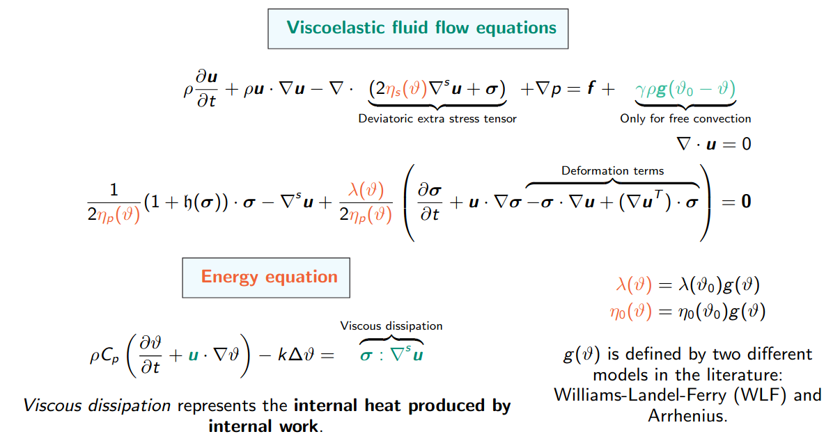
where \(\theta\) is the temperature unknown and \(\theta_0\) is the referene temperature.
To solve the full problem, we use an iterative coupling strategy between the thermal and fluid subproblems, while the fluid equations are treated in a monolithic way, that is, solved all together rather than split into separate steps.
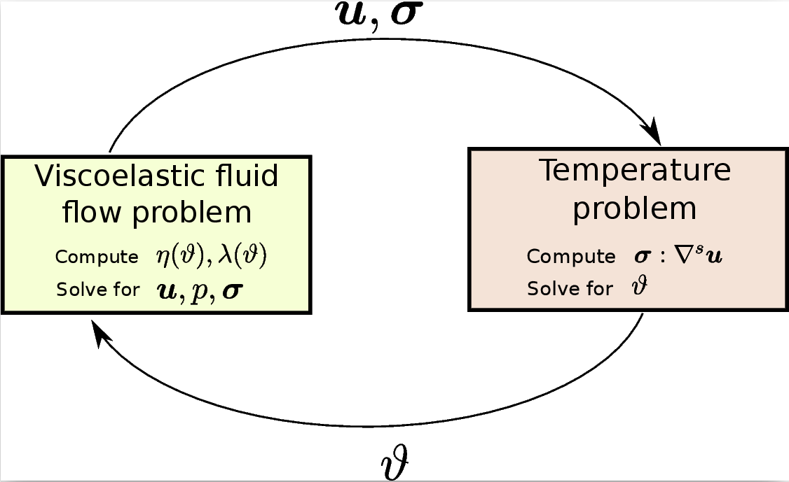
As in the previous section, we rely on the Split-OSS stabilization technique for all numerical simulations, and the LCR formulation is also coupled in order to capture more elastic behaviors (see Log-Conformation Reformulation Section for more details).
4.2 Numerical Results
Flow around a cylinder
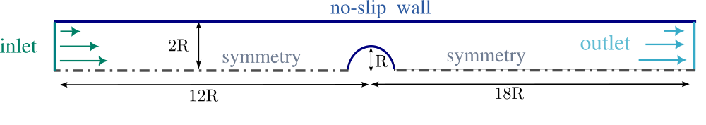
This benchmark isn’t the most exciting one, but it is widely used to test numerical formulations. Moreover, it’s a solid and well-understood setup for evaluating how different methods perform when simulating viscoelastic fluid flows, and it remains useful for validating models under both isothermal and non-isothermal conditions. Only the half of the channel was considered due to the symmetry nature of the test.
All the details about the material properties, boundary conditions, and mesh employed are included in the paper. Regarding the results, we have studied the role that viscoelasticity plays in the temperature distribution of the fluid flow. The next picture shows the temperature distribution along the channel.
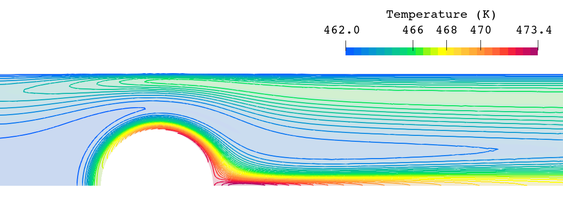
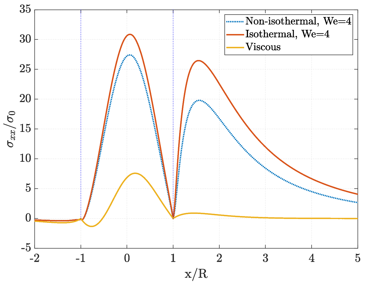
We can observe that the temperature increases around the cylinder and downstream when considering a fluid flow with \(\text{We}= 4\). Now we can also compare the behaviour of the temperature for fluid flows with different viscoelasticity (different We), and also comparing with a viscous fluid flow.
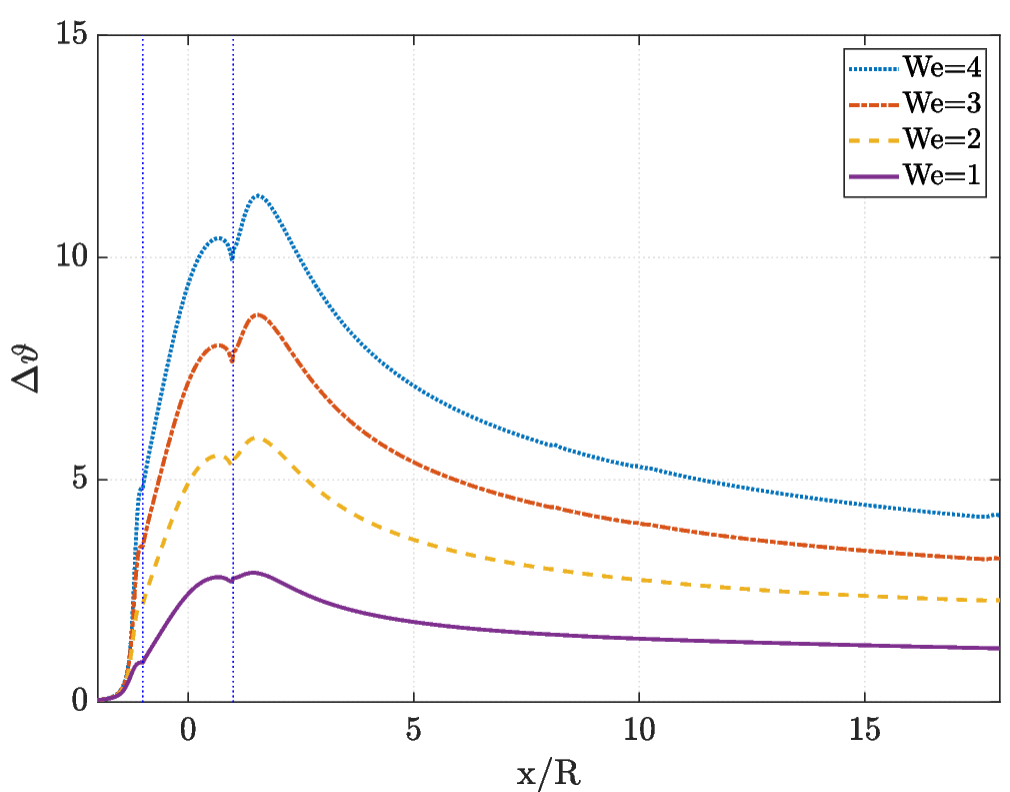
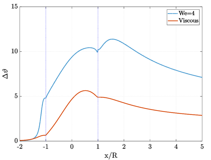
From these results, we can conclude that viscoelastic fluid flow generates heat in areas with higher viscous dissipation. Another important finding concerns the stresses (again, over the cylinder and downstream): when viscoelasticity is coupled with the temperature equation, the stress values decrease significantly.
I strongly recommend checking the other example in the paper (“extension 1:3”), where we observed a bifurcation at high Reynolds numbers. It’s a rich and interesting case, where we studied how variations in four dimensionless numbers (Reynolds, Weissenberg, Prandtl, and Bingham) affect the flow behaviour. Additionally tests were performed with highly elastic fluids.
4.3 Conclusions
The coupling of viscoelastic fluids with temperature allows us to understand how these fluids heat up, which occurs differently compared to purely viscous fluids. Understanding these temperature distributions can be very beneficial for replicating various industrial processes, making this study particularly relevant. What do you think? Are you familiar with how elasticity can affect temperature in fluid flows?
5 Time-dependent subgrid-scales
In construction.
6 Purely elastic inestability and Fractional Step Methods
In construction.
7 Fluid-Structure Interaction
In construction.
8 Numerical Analysis
In construction.
This research line formed the core of my PhD thesis, defended at the Universitat Politècnica de Catalunya (UPC).